PLEQUE vs raw reconstruction

In this notebook, we demonstrate that PLEQUE is better than raw reconstruction at everything.

%pylab inline

Populating the interactive namespace from numpy and matplotlib

from pleque.io import _geqdsk as eqdsktool
from pleque.io.readers import read_geqdsk
from pleque.utils.plotting import *
#from pleque import Equilibrium
from pleque.tests.utils import get_test_equilibria_filenames, load_testing_equilibrium

Load a testing equilibrium

Several test equilibria come shipped with PLEQUE. Their location is:

gfiles = get_test_equilibria_filenames()
gfiles

['/home/docs/checkouts/readthedocs.org/user_builds/pleque/envs/develop/lib/python3.6/site-packages/pleque/resources/baseline_eqdsk',
 '/home/docs/checkouts/readthedocs.org/user_builds/pleque/envs/develop/lib/python3.6/site-packages/pleque/resources/scenario_1_baseline_upward_eqdsk',
 '/home/docs/checkouts/readthedocs.org/user_builds/pleque/envs/develop/lib/python3.6/site-packages/pleque/resources/DoubleNull_eqdsk',
 '/home/docs/checkouts/readthedocs.org/user_builds/pleque/envs/develop/lib/python3.6/site-packages/pleque/resources/g13127.1050',
 '/home/docs/checkouts/readthedocs.org/user_builds/pleque/envs/develop/lib/python3.6/site-packages/pleque/resources/14068@1130_2kA_modified_triang.gfile',
 '/home/docs/checkouts/readthedocs.org/user_builds/pleque/envs/develop/lib/python3.6/site-packages/pleque/resources/g15349.1120',
 '/home/docs/checkouts/readthedocs.org/user_builds/pleque/envs/develop/lib/python3.6/site-packages/pleque/resources/shot8078_jorek_data.nc']

Load the equilibrium directly

Here the test equilibrium is directly loaded and stored in the variable eq_efit. The variable then contains all equilibrium information calculated by EFIT in the form of a dictionary.

test_case_number = 5

with open(gfiles[test_case_number], 'r') as f:
    eq_efit = eqdsktool.read(f)
eq_efit.keys()

  nx = 33, ny = 33
361 231

dict_keys(['nx', 'ny', 'rdim', 'zdim', 'rcentr', 'rleft', 'zmid', 'rmagx', 'zmagx', 'simagx', 'sibdry', 'bcentr', 'cpasma', 'F', 'pres', 'FFprime', 'pprime', 'psi', 'q', 'rbdry', 'zbdry', 'rlim', 'zlim'])

Load equilibrium using PLEQUE

PLEQUE loads the same file at its core, but it wraps it in the Equilibrium class and stores it in the variable eq.

def save_it(*args,**kwargs):
    pass

#Load equilibrium stored in the EQDSK format
eq = read_geqdsk(gfiles[test_case_number])

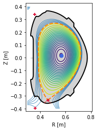
#Plot basic overview of the equilibrium
plt.figure()
eq._plot_overview()

#Plot X-points
plot_extremes(eq, markeredgewidth=2)

  nx = 33, ny = 33
361 231

PLEQUE vs raw reconstruction: spatial resolution near the X-point

EFIT output (\(\Psi\), \(j\) etc.) is given on a rectangular grid:

r_axis = np.linspace(eq_efit["rleft"], eq_efit["rleft"] + eq_efit["rdim"], eq_efit["nx"])
z_axis = np.linspace(eq_efit["zmid"] - eq_efit["zdim"] / 2, eq_efit["zmid"] + eq_efit["zdim"] / 2, eq_efit["ny"])

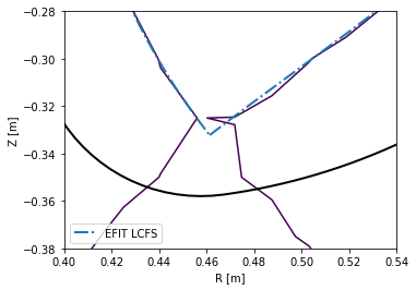
To limit the file size, the grid has a finite resolution. This means that in areas where high spatial resolution is needed (for instance the X-point vicinity), raw reconstructions are usually insufficient. The following figure demonstrates this.

plt.figure()
ax = plt.gca()

#Limiter (stored in EFIT output)
ax.plot(eq_efit['rlim'], eq_efit['zlim'], color='k', lw=2)

#Magnetic surface defined by Psi == eq_efit['sibdry']
ax.contour(r_axis, z_axis, eq_efit['psi'].T, [eq_efit['sibdry']])

#Magnetic surface saved as the LCFS in EFIT output
ax.plot(eq_efit['rbdry'], eq_efit['zbdry'], 'C0-.', lw=2, label='EFIT LCFS')

ax.set_xlabel('R [m]')
ax.set_ylabel('Z [m]')
ax.set_aspect('equal')
plt.legend()
ax.set_xlim(0.4, 0.54)
ax.set_ylim(-0.38, -0.28)

(-0.38, -0.28)

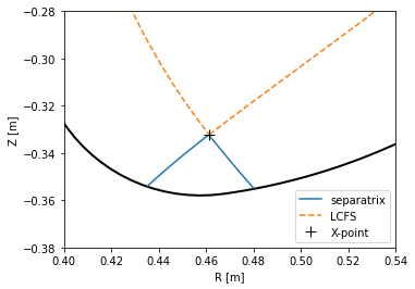
PLEQUE, however, performs equilibrium interpolation that can easily produce the same plots in a much higher spatial resolution.

plt.figure()
ax = plt.gca()

#Limiter (accessed through the Equilibrium class)
eq.first_wall.plot(ls="-", color="k", lw=2)

#Separatrix, cropped to its part inside the first wall
inside_fw = eq.in_first_wall(eq.separatrix)
separatrix = eq.coordinates(R=eq.separatrix.R[inside_fw], Z=eq.separatrix.Z[inside_fw])
separatrix.plot(label='separatrix')

#LCFS (without strike points)
eq.lcfs.plot(color='C1', ls='--', label='LCFS')

#X-point
ax.plot(eq._x_point[0], eq._x_point[1], 'k+', markersize=10, label='X-point')

ax.set_xlabel('R [m]')
ax.set_ylabel('Z [m]')
ax.set_aspect('equal')
plt.legend()
ax.set_xlim(0.4, 0.54)
ax.set_ylim(-0.38, -0.28)

(-0.38, -0.28)

PLEQUE vs raw reconstruction: \(q\) profile

The safety factor \(q\) can be defined as the number of toroidal turns a magnetic field line makes along its magnetic surface before it makes a full poloidal turn. Since the poloidal field is zero at the X-point, the magnetic field lines inside the separatrix are caught in an infinite toroidal loop at the X-point and \(q \rightarrow +\infty\). (This is why the edge safety factor is given as \(q_{95}\) at \(\psi_N=0.95\). If it were given an \(\psi_N = 1.00\), its value would diverge regardless of its profile shape.)

In this section we compare several methods of calculating \(q\):

1. \(q\) as calculated by the reconstruction itself (q_efit)
2. \(q\) evaluated by eq.q (q_eq)
3. \(q\) evaluated by eq._flux_surface(psi_n).eval_q
   • using the default, rectangle rule (q1)
   • using the trapezoidal rule (q2)
   • using the Simpson rule (q3)

Method 3 calculates the safety factor according to formula (5.35) in [Jardin, 2010: Computation Methods in Plasma Physics]:

\(q(\psi) = \dfrac{gV'}{(2\pi)^2\Psi'}\langle R^{-2}\rangle\)

where \(V'\) is the differential volume and, in PLEQUE’s notation, \(g(\psi) \equiv F(\psi)\) and \(\Psi \equiv \psi\) (and therefore \(\Psi' \equiv d\Psi/d\psi = 1\)). Furthermore, the surface average \(\langle \cdot \rangle\) of an arbitrary function \(a\) is defined as \(\langle a \rangle = \frac{2\pi}{V'} \int_0^{2\pi} d\theta Ja\) where \(J\) is the Jacobian. Putting everything together, one obtains the formula used by PLEQUE:

\(q(\psi) = \dfrac{F(\psi)}{2\pi} \int_0^{2\pi} d\theta JR^{-2}\)

where, based on the convention defined by COCOS, the factor \(2\pi\) can be missing and \(q\) may be either positive or negative. (In the default convention of EFIT, COCOS 3, \(q\) is negative.) Finally, the integral can be calculated with three different methods: the rectangle rule (resulting in q1), the trapezoidal rule (resulting in q2) and the Simpson rule (resulting in q3).

Method 2 is based on method 3. The safety factor profile is calculated for 200 points in \(\psi_N \in (0, 1)\) and interpolated with a spline. eq.q then invokes this spline to calculate \(q\) at any given \(\psi_N\).

#q taken directly from the reconstruction
q_efit = eq_efit['q']
q_efit = q_efit[:-1] #in some reconstructions, q is calculated up to psi_N=1
psi_efit = np.linspace(0, 1, len(q_efit), endpoint=False)
#psi_efit2 = np.linspace(0, 1, len(q_efit), endpoint=True)
# If you try this for several test equilibria, you will find that some give q at Psi_N=1
# and some stop right short of Psi_N=1. To test which is which, try both including and
# excluding the endpoint in the linspace definition.

#q stored in the Equilibrium class
coords = eq.coordinates(psi_n = np.linspace(0, 1, len(q_efit), endpoint=False))
psi_eq = coords.psi_n
q_eq = abs(eq.q(coords))

#q calculated by eq._flux_surface(Psi).eval_q
surf_psin = linspace(0.01, 1, len(q_efit), endpoint=False)
surfs = [eq._flux_surface(psi_n=psi_n)[0] for psi_n in surf_psin]
surf_psin = [np.mean(s.psi_n) for s in surfs]
q1 = abs(np.array([np.asscalar(s.eval_q) for s in surfs]))
q2 = abs(np.array([np.asscalar(s.get_eval_q('trapz')) for s in surfs]))
q3 = abs(np.array([np.asscalar(s.get_eval_q('simps')) for s in surfs]))

/home/docs/checkouts/readthedocs.org/user_builds/pleque/envs/develop/lib/python3.6/site-packages/ipykernel_launcher.py:19: DeprecationWarning: np.asscalar(a) is deprecated since NumPy v1.16, use a.item() instead
/home/docs/checkouts/readthedocs.org/user_builds/pleque/envs/develop/lib/python3.6/site-packages/ipykernel_launcher.py:20: DeprecationWarning: np.asscalar(a) is deprecated since NumPy v1.16, use a.item() instead
/home/docs/checkouts/readthedocs.org/user_builds/pleque/envs/develop/lib/python3.6/site-packages/ipykernel_launcher.py:21: DeprecationWarning: np.asscalar(a) is deprecated since NumPy v1.16, use a.item() instead

Notice the absolute value; this is required because \(q<0\) in the convention used here.

#q profile comparison
plt.figure()
plt.plot(psi_efit, q_efit, 'x', label='raw reconstruction')
#plt.plot(psi_efit2, q_efit, 'x', label='raw reconstruction')
plt.plot(psi_eq, q_eq, '--', label=r'pleque: eq.q')
plt.plot(surf_psin, q1, '-', label=r'pleque: q1')
plt.plot(surf_psin, q2, '--', label=r'pleque: q2')
plt.plot(surf_psin, q3, '--', label=r'pleque: q3')
plt.xlabel(r'$\psi_\mathrm{N}$')
plt.ylabel(r'$q$')
plt.axvline(1, ls='--', color='k', lw=1)
plt.legend()

<matplotlib.legend.Legend at 0x7f4fe00405c0>

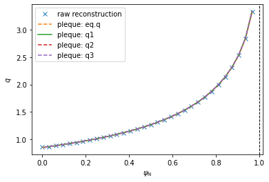
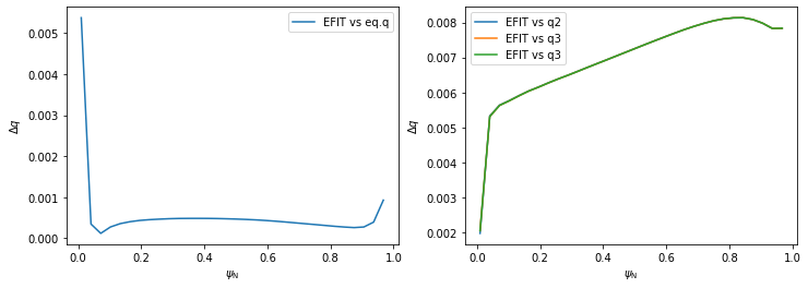
Investigating the differences between the five \(q\) profiles shows quite a good agreement. The profiles disagree slightly near \(\psi_N \rightarrow 0\) since the safety factor is defined by a limit here. (Notice that, using method 3, the \(\psi_N\) axis begins at 0.01 and not 0. This is because \(q\) cannot be calculated by the formula above in \(\psi_N=0\) and the algorithm fails.)

plt.figure(figsize=(12,4))

#EFIT vs eq.q
plt.subplot(121)
plt.plot(surf_psin, abs(q_eq-q_efit), label='EFIT vs eq.q')
plt.legend()
plt.xlabel(r'$\psi_\mathrm{N}$')
plt.ylabel(r'$\Delta q$')

#EFIT vs q1-q3
plt.subplot(122)
plt.plot(surf_psin, abs(q_efit-q1), label='EFIT vs q2')
plt.plot(surf_psin, abs(q_efit-q2), label='EFIT vs q3')
plt.plot(surf_psin, abs(q_efit-q3), label='EFIT vs q3')
plt.legend()
plt.xlabel(r'$\psi_\mathrm{N}$')
plt.ylabel(r'$\Delta q$')


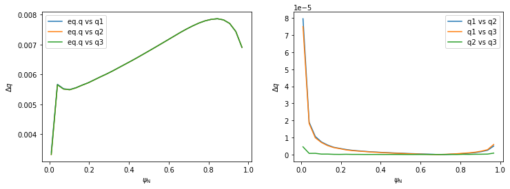
plt.figure(figsize=(12,4))

#eq.q vs all the rest
plt.subplot(121)
plt.plot(surf_psin, abs(q_eq-q1), label='eq.q vs q1')
plt.plot(surf_psin, abs(q_eq-q2), label='eq.q vs q2')
plt.plot(surf_psin, abs(q_eq-q3), label='eq.q vs q3')
plt.legend()
plt.xlabel(r'$\psi_\mathrm{N}$')
plt.ylabel(r'$\Delta q$')

#q1 vs q2 vs q3
plt.subplot(122)
plt.plot(surf_psin, abs(q1-q2), label='q1 vs q2')
plt.plot(surf_psin, abs(q1-q3), label='q1 vs q3')
plt.plot(surf_psin, abs(q2-q3), label='q2 vs q3')
plt.legend()
plt.xlabel(r'$\psi_\mathrm{N}$')
plt.ylabel(r'$\Delta q$')

Text(0, 0.5, '$\\Delta q$')

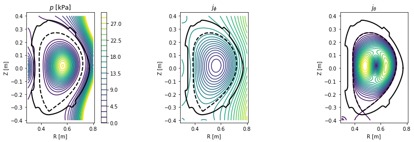
Plotting contour plots of various quantities

In this section PLEQUE is used to produce contour plots of the following quantities:

• poloidal magnetic field flux \(\psi\)
• toroidal magnetic field flux
• poloidal magnetic field \(B_p\)
• toroidal magnetic field \(B_t\)
• total magnetic field \(|B|\)
• total pressure \(p\)
• toroidal current density \(j_\phi\)
• poloidal current density \(j_\theta\)

First, a general plotting function plot_2d is defined.

def plot_2d(R, Z, data, *args, title=None):

    #Define X and Y axis limits based on the vessel size
    rlim = [np.min(eq.first_wall.R), np.max(eq.first_wall.R)]
    zlim = [np.min(eq.first_wall.Z), np.max(eq.first_wall.Z)]
    size = rlim[1] - rlim[0]
    rlim[0] -= size / 12
    rlim[1] += size / 12
    size = zlim[1] - zlim[0]
    zlim[0] -= size / 12
    zlim[1] += size / 12

    #Set up the figure: set axis limits, draw LCFS and first wall, write labels
    ax = plt.gca()
    ax.set_xlim(rlim)
    ax.set_ylim(zlim)
    ax.plot(eq.lcfs.R, eq.lcfs.Z, color='k', ls='--', lw=2)
    ax.plot(eq.first_wall.R, eq.first_wall.Z, 'k-', lw=2)
    ax.set_xlabel('R [m]')
    ax.set_ylabel('Z [m]')
    ax.set_aspect('equal')
    if title is not None:
        ax.set_title(title)

    #Finally, plot the desired quantity
    cl = ax.contour(R, Z, data, *args)

    return cl

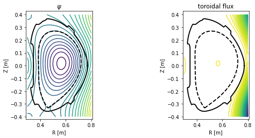
Now we set up an \([R,Z]\) grid where these quantities are evaluated and plot the quantities.

#Create an [R,Z] grid 200 by 300 points
grid = eq.grid((200,300), dim='size')

#Plot the poloidal flux and toroidal flux
plt.figure(figsize=(16,4))
plt.subplot(131)
plot_2d(grid.R, grid.Z, grid.psi, 20, title=r'$\psi$')
plt.subplot(132)
plot_2d(grid.R, grid.Z, eq.tor_flux(grid), 100, title='toroidal flux')

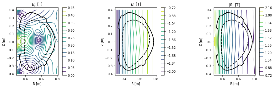
#Plot the poloidal magnetic field, toroidal magnetic field and the total magnetic field
plt.figure(figsize=(16,4))
plt.subplot(131)
cl = plot_2d(grid.R, grid.Z, eq.B_pol(grid), 20, title=r'$B_\mathrm{p}$ [T]')
plt.colorbar(cl)
plt.subplot(132)
cl = plot_2d(grid.R, grid.Z, eq.B_tor(grid), 20, title=r'$B_\mathrm{t}$ [T]')
plt.colorbar(cl)
plt.subplot(133)
cl = plot_2d(grid.R, grid.Z, eq.B_abs(grid), 20, title=r'$|B|$ [T]')
plt.colorbar(cl)

#Plot the total pressure, toroidal current density and poloidal current density
plt.figure(figsize=(16,4))
plt.subplot(131)
cl = plot_2d(grid.R, grid.Z, eq.pressure(grid)/1e3, np.linspace(0, 30, 21), title=r'$p$ [kPa]')
plt.colorbar(cl)
plt.subplot(132)
plot_2d(grid.R, grid.Z, eq.j_tor(grid), np.linspace(-5e6, 5e6, 30), title=r'$j_\phi$')
plt.subplot(133)
plot_2d(grid.R, grid.Z, eq.j_pol(grid),  np.linspace(0, 3e5, 21), title=r'$j_\theta$')

<matplotlib.contour.QuadContourSet at 0x7f4fdf6daba8>

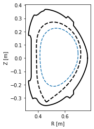
Exploring flux surface properties

With the eq._flux_surface(psi_n) function, one may study individual flux surfaces. In this section, we plot the \(\psi_N=0.8\) flux surface and calculate its safety factor \(q\), length in the poloidal direction, total 3D area, volume and toroidal current density.

#Define the flux surface by its normalised poloidal flux
surf = eq._flux_surface(psi_n=0.8)[0]

#Plot the flux surface
plt.figure()
ax = gca()
ax.plot(eq.lcfs.R, eq.lcfs.Z, color='k', ls='--', lw=2)
ax.plot(eq.first_wall.R, eq.first_wall.Z, 'k-', lw=2)
surf.plot(ls='--')
ax.set_xlabel('R [m]')
ax.set_ylabel('Z [m]')
ax.set_aspect('equal')

#Calculate several flux surface quantities
print('Safety factor: %.2f' % surf.eval_q[0])
print('Length: %.2f m' % surf.length)
print('Area: %.4f m^2' % surf.area)
print('Volume: %.3f m^3' % surf.volume)
print('Toroidal current density: %.3f MA/m^2' % (surf.tor_current/1e6))

Safety factor: -1.94
Length: 1.16 m
Area: 0.0989 m^2
Volume: 0.339 m^3
Toroidal current density: -0.213 MA/m^2

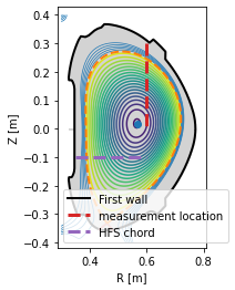
Profile mapping

In experiment one often encounters the need to compare profiles which were measured at various locations in the tokamak. In this section, we show how such a profile may be mapped onto an arbitrary location and to the outer midplane.

The profile is measured at the plasma top (in red) and mapped to the HFS (in violet) and the outer midplane (not shown).

#Define the chord along which the profile was measured (in red)
N = 200 #number of datapoints in the profile
chord = eq.coordinates(R=0.6*np.ones(N), Z=np.linspace(0.3, 0., N))

#Define the HFS chord where we wish to map the profile (in violet)
chord_hfs = eq.coordinates(R=np.linspace(0.35, 0.6, 20), Z=-0.1*np.ones(20))

#Plot both the chords
plt.figure()
eq._plot_overview()
chord.plot(lw=3, ls='--', color='C3', label='measurement location')
chord_hfs.plot(lw=3, ls='--', color='C4', label='HFS chord')
plt.legend(loc=3)

<matplotlib.legend.Legend at 0x7f4fdf7b7c50>

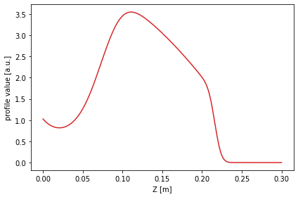
The profile shape is defined using the error function erf.

from scipy.special import erf

#Define the profile values
prof_func = lambda x, k1, xsep: k1/4 * (1 + erf((x-xsep)*20))*np.log((x+1)*1.2) - 4*np.exp(-(50*(x-1)**2))
profile = prof_func(1 - chord.psi_n, 10, 0.15)

#Plot the profile along the chord it was measured at
plt.figure()
plt.plot(chord.Z, profile, color='C3')
plt.xlabel('Z [m]')
plt.ylabel('profile value [a.u.]')
plt.tight_layout()

To begin the mapping, the profile is converted into a flux function by eq.fluxfuncs.add_flux_func(). The flux function is a spline, and therefore it can be evaluated at any \(\psi_N\) coordinate covered by the original chord. This will allow its mapping to any other coordinate along the flux surfaces.

eq.fluxfuncs.add_flux_func('test_profile', profile, chord, spline_smooth=0)

<scipy.interpolate.fitpack2.InterpolatedUnivariateSpline at 0x7f4fdf916c18>

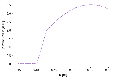
To evaluate the flux function along a chord, simply pass the chord (an instance of the Coordinates class) to the flux function. In the next figure the profile is mapped to the HFS cord.

#Map the profile to the HFS cord
plt.figure()
plt.plot(chord_hfs.R, eq.fluxfuncs.test_profile(chord_hfs), '--', color='C4')
plt.xlabel('R [m]')
plt.ylabel('profile value [a.u.]')

Text(0, 0.5, 'profile value [a.u.]')

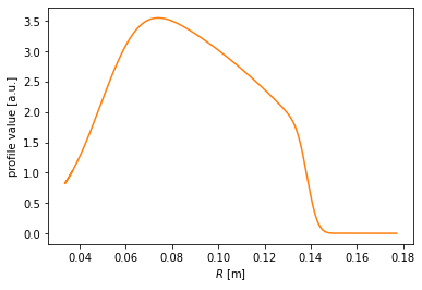
For the outer midplane, no special chord need be specified. Every instance of the Coordinates class can automatically map its coordinates to the outer midplane. (Note that this doesn’t require a flux function to be specified. The conversion is performed in the coordinates only.)

#Map the profile to the outer midplane
plt.figure()
plt.plot(chord.r_mid, profile, color='C1')
plt.xlabel(r'$R$ [m]')
plt.ylabel('profile value [a.u.]')

Text(0, 0.5, 'profile value [a.u.]')

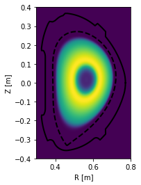
Finally, the profile may be drawn along the entire poloidal cross section.

#Assuming poloidal symmetry, plot the profile in the poloidal cross section
plt.figure()
ax = gca()
ax.plot(eq.lcfs.R, eq.lcfs.Z, color='k', ls='--', lw=2)
ax.plot(eq.first_wall.R, eq.first_wall.Z, 'k-', lw=2)
grid = eq.grid()
ax.pcolormesh(grid.R, grid.Z, eq.fluxfuncs.test_profile(grid))
ax.set_xlabel('R [m]')
ax.set_ylabel('Z [m]')
ax.set_aspect('equal')

/home/docs/checkouts/readthedocs.org/user_builds/pleque/envs/develop/lib/python3.6/site-packages/ipykernel_launcher.py:7: MatplotlibDeprecationWarning: shading='flat' when X and Y have the same dimensions as C is deprecated since 3.3.  Either specify the corners of the quadrilaterals with X and Y, or pass shading='auto', 'nearest' or 'gouraud', or set rcParams['pcolor.shading'].  This will become an error two minor releases later.
  import sys

Detector line of sight visualisation

In this section, we demonstrate the flexibility of the Coordinates class by visualising a detector line of sight. Suppose we have a pixel detector at the position \([X, Y, Z] = [1.2 \, \mathrm{m}, 0 \, \mathrm{m}, -0.1 \, \mathrm{m}]\).

# Define detector position [X, Y, Z]
position = np.array((1.2, 0, -0.1))

The detector views the plasma mostly tangentially to the toroidal direction, but also sloping a little upward.

#Define the line of sight direction (again along [X, Y, Z])
direction = np.array((-1, 0.6, 0.2))

#Norm the direction to unit length
direction /= np.linalg.norm(direction)

Now since the plasma geometry is curvilinear, the detector line of sight is not trivial. Luckily PLEQUE’s Coordinates class can easily express its stored coordinates both in the cartesian \([X,Y,Z]\) and the cylindrical \([R,Z,\phi]\) coordinate systems. In the following line, 20 points along the detector line of sight are calculated in 3D.

# Calculate detector line of sight (LOS)
LOS = eq.coordinates(position + direction[np.newaxis,:] * np.linspace(0, 2.0, 20)[:, np.newaxis],
                     coord_type=('X', 'Y', 'Z')
                    )

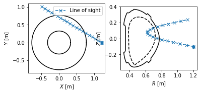
To visualise the line of sight in top view \([X,Y]\) and poloidal cross-section view \([R,Z]\), we first define the limiter outline as viewed from the top. Then we proceed with the plotting.

# Limiter outline viewed from the top
Ns = 100
inner_lim = eq.coordinates(np.min(eq.first_wall.R)*np.ones(Ns), np.zeros(Ns), np.linspace(0, 2*np.pi, Ns))
outer_lim = eq.coordinates(np.max(eq.first_wall.R)*np.ones(Ns), np.zeros(Ns), np.linspace(0, 2*np.pi, Ns))

# Prepare figure
fig, axs = plt.subplots(1,2)

# Top view
ax = axs[0]
ax.plot(inner_lim.X, inner_lim.Y, 'k-')
ax.plot(outer_lim.X, outer_lim.Y, 'k-')
ax.plot(LOS.X, LOS.Y, 'x--', label='Line of sight')
ax.plot(position[0], position[1], 'd', color='C0')
ax.legend()
ax.set_aspect('equal')
ax.set_xlabel('$X$ [m]')
ax.set_ylabel('$Y$ [m]')

# Poloidal cross-section view
ax = axs[1]
ax.plot(eq.first_wall.R, eq.first_wall.Z, 'k-')
ax.plot(eq.lcfs.R, eq.lcfs.Z, 'k--')
ax.plot(LOS.R, LOS.Z, 'x--')
ax.plot(LOS.R[0], position[2], 'd', color='C0')
ax.set_aspect('equal')
ax.set_xlabel('$R$ [m]')
ax.set_ylabel('$Z$ [m]')

Text(0, 0.5, '$Z$ [m]')

Field line tracing

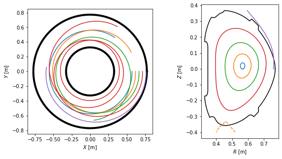
In this section, we show how to trace field lines and calculate their length. (In the core plasma, the length is defined as the parallel distance of one poloidal turn. In the SOL, it’s the so-called connection length.) First we define a set of five starting points, all located at the outer midplane (\(Z=0\)) with \(R\) going from \(0.55 \, \mathrm{m}\) (core) to \(0.76\, \mathrm{m}\) (SOL).

# Define the starting points
N = 5
Rs = np.linspace(0.57, 0.76, N, endpoint=True)
Zs = np.zeros_like(Rs)

Next, the field lines beginning at these points are traced. The default tracing direction is direction=1, that is, following the direction of the toroidal magnetic field.

traces = eq.trace_field_line(R=Rs, Z=Zs)

direction: 1
dphidtheta: 1.0
direction: 1
dphidtheta: 1.0
direction: 1
dphidtheta: 1.0
direction: 1
dphidtheta: 1.0

To visualise the field lines, we plot them in top view, poloidal cross-section view and 3D view.

# Define limiter as viewed from the top
Ns = 100
inner_lim = eq.coordinates(np.min(eq.first_wall.R)*np.ones(Ns), np.zeros(Ns), np.linspace(0, 2*np.pi, Ns))
outer_lim = eq.coordinates(np.max(eq.first_wall.R)*np.ones(Ns), np.zeros(Ns), np.linspace(0, 2*np.pi, Ns))

fig = plt.figure(figsize=(10,5))

#Plot top view of the field lines
ax = plt.subplot(121)
plt.plot(inner_lim.X, inner_lim.Y, 'k-', lw=4)
plt.plot(outer_lim.X, outer_lim.Y, 'k-', lw=4)
for fl in traces:
    ax.plot(fl.X, fl.Y)
ax.set_xlabel('$X$ [m]')
ax.set_ylabel('$Y$ [m]')
ax.set_aspect('equal')

#Plot poloidal cross-section view of the field lines
ax = plt.subplot(122)
plt.plot(eq.first_wall.R, eq.first_wall.Z, 'k-')
plt.plot(eq.separatrix.R, eq.separatrix.Z, 'C1--')
for fl in traces:
    plt.plot(fl.R, fl.Z)
ax.set_xlabel('$R$ [m]')
ax.set_ylabel('$Z$ [m]')
ax.set_aspect('equal')

#Plot 3D view of the field lines
from mpl_toolkits.mplot3d import Axes3D
fig = plt.figure(figsize=(6,6))
ax = fig.gca(projection='3d')
for fl in traces:
    ax.scatter(fl.X, fl.Y, fl.Z, s=0.3, marker='.')
ax.set_xlabel('$X$ [m]')
ax.set_ylabel('$Y$ [m]')
ax.set_zlabel('$Z$ [m]')
#ax.set_aspect('equal')

Text(0.5, 0, '$Z$ [m]')

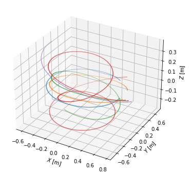
One may calculate the field line length using the attribute length. To demonstrate the connection length profile, we define a couple more SOL field lines. Note that now the direction argument changes whether we trace to the HFS or LFS limiter/divertor. Also pay attention to the in_first_wall=True argument, which tells the field lines to terminate upon hitting the first wall. (Otherwise they would be terminated at the edge of a rectangle surrounding the vacuum vessel.)

Rsep = 0.7189 # You might want to change this when switching between different test equilibria.
Rs_SOL = Rsep + 0.001*np.array([0, 0.2, 0.5, 0.7, 1, 1.5, 2.5, 4, 6, 9, 15, 20])
Zs_SOL = np.zeros_like(Rs_SOL)

SOL_traces = eq.trace_field_line(R=Rs_SOL, Z=Zs_SOL, direction=-1, in_first_wall=True)

Finally we calculate the connection length and plot its profile.

#Calculate field line length
L = np.array([traces[k].length for k in range(N)])
L_conn = np.array([SOL_traces[k].length for k in range(len(SOL_traces))])

fig = plt.figure(figsize=(10,5))

#Plot poloidal cross-section view of the field lines
ax = plt.subplot(121)
ax.plot(eq.first_wall.R, eq.first_wall.Z, 'k-')
ax.plot(eq.separatrix.R, eq.separatrix.Z, 'C1--')
for fl in np.hstack((traces, SOL_traces)):
    ax.plot(fl.R, fl.Z)
ax.set_xlabel('R [m]')
ax.set_ylabel('Z [m]')
ax.set_aspect('equal')

#Plot connection length profile
ax = plt.subplot(122)
ax.plot(Rs, L, 'bo')
ax.plot(Rs_SOL, L_conn, 'ro')
ax.set_xlabel('R [m]')
ax.set_ylabel('L [m]')

Text(0, 0.5, 'L [m]')

Straight field lines

In the field of MHD, it is sometimes advantageous to go from the normal toroidal coordinates \([R, \theta, \phi]\) to a coordinate system \([R, \theta^*, \phi]\) where field lines are straight. In this section, we show how to define such a coordinate system using PLEQUE.

The field line we are going to visualise is on the resonant surface \(q=5/3\) (and therefore it closes upon itself after three poloidal turns). First, we find the \(\Psi_N\) of this surface.

from scipy.optimize import minimize_scalar, brentq

#Find the Psi_N where the safety factor is 5/3
psi_onq = brentq(lambda psi_n: np.abs(eq.q(psi_n)) - 5/3, 0, 0.95)
print(r'Psi_N = {:.3f}'.format(psi_onq))

#Define the resonant flux surface using this Psi_N
surf = eq._flux_surface(psi_n = psi_onq)[0]

Psi_N = 0.714

from scipy.interpolate import CubicSpline
from numpy import ma #module for masking arrays

#Define the normal poloidal coordinate theta (and subtract 2*pi from any value that exceeds 2*pi)
theta = np.mod(surf.theta, 2*np.pi)

#Define the special poloidal coordinate theta_star and
theta_star = surf.straight_fieldline_theta

#Sort the two arrays to start at theta=0 and decrease their spatial resolution by 75 %
asort = np.argsort(theta)
#should be smothed
theta = theta[asort][2::4]
theta_star = theta_star[asort][2::4]

#Interpolate theta_star with a periodic spline
thstar_spl = CubicSpline(theta, theta_star, extrapolate='periodic')

Now we trace a field line along the resonant magnetic surface, starting at the midplane (the intersection of the resonant surface with the horizontal plane passing through the magnetic axis). Since the field line is within the confined plasma, the tracing terminates after one poloidal turn. We begin at the last point of the field line and restart the tracing two more times, obtaining a full field line which closes into itself.

tr1 = eq.trace_field_line(r=eq.coordinates(psi_onq).r_mid[0], theta=0.09)[0]
tr2 = eq.trace_field_line(tr1.R[-1], tr1.Z[-1], tr1.phi[-1])[0]
tr3 = eq.trace_field_line(tr2.R[-1], tr2.Z[-1], tr2.phi[-1])[0]

direction: 1
dphidtheta: 1.0
direction: 1
dphidtheta: 1.0
direction: 1
dphidtheta: 1.0

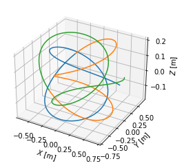
We visualise the field lines in top view, poloidal cross-section view and 3D view. Notice that the field lines make five toroidal turns until they close in on themselves, which corresponds to the \(m=5\) resonant surface.

plt.figure(figsize=(10,5))

# Define limiter as viewed from the top
Ns = 100
inner_lim = eq.coordinates(np.min(eq.first_wall.R)*np.ones(Ns), np.zeros(Ns), np.linspace(0, 2*np.pi, Ns))
outer_lim = eq.coordinates(np.max(eq.first_wall.R)*np.ones(Ns), np.zeros(Ns), np.linspace(0, 2*np.pi, Ns))

#Plot the field lines in top view
ax = plt.subplot(121)
ax.plot(inner_lim.X, inner_lim.Y, 'k-', lw=4)
ax.plot(outer_lim.X, outer_lim.Y, 'k-', lw=4)
ax.plot(tr1.X, tr1.Y)
ax.plot(tr2.X, tr2.Y)
ax.plot(tr3.X, tr3.Y)
ax.set_xlabel('$X$ [m]')
ax.set_ylabel('$Y$ [m]')
ax.set_aspect('equal')

#Plot the field lines in the poloidal cross-section view
ax = plt.subplot(122)
ax.plot(eq.first_wall.R, eq.first_wall.Z, 'k-')
ax.plot(eq.lcfs.R, eq.lcfs.Z, 'k--')
ax.plot(tr1.R, tr1.Z)
ax.plot(tr2.R, tr2.Z)
ax.plot(tr3.R, tr3.Z)
ax.set_xlabel('$R$ [m]')
ax.set_ylabel('$Z$ [m]')
ax.set_aspect('equal')

#Plot the field line in 3D
fig = plt.figure()
ax = fig.gca(projection='3d')
ax.plot(tr1.X, tr1.Y, tr1.Z)
ax.plot(tr2.X, tr2.Y, tr2.Z)
ax.plot(tr3.X, tr3.Y, tr3.Z)
#ax.set_aspect('equal')
ax.set_xlabel('$X$ [m]')
ax.set_ylabel('$Y$ [m]')
ax.set_zlabel('$Z$ [m]')

Text(0.5, 0, '$Z$ [m]')

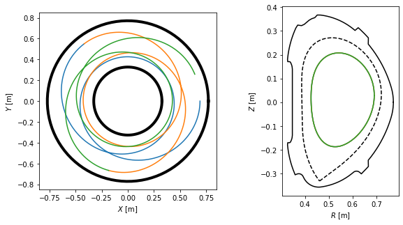
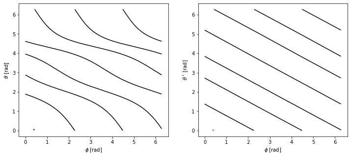
Plotting the field lines in the \([\theta, \phi]\) and \([\theta^*, \phi]\) coordinates, we find that they are curves in the former and straight lines in the latter.

fig, axes = plt.subplots(1, 2, figsize=(12,5))
ax1, ax2 = axes

for t in [tr1, tr2, tr3]:
    # Extract the theta, theta_star and Phi coordinates from the field lines
    theta = np.mod(t.theta, 2*np.pi)
    theta_star = thstar_spl(theta)
    phi = np.mod(t.phi, 2*np.pi)

    # Mask the coordinates for plotting purposes
    theta = ma.masked_greater(theta, 2*np.pi-1e-2)
    theta = ma.masked_less(theta, 1e-2)
    theta_star = ma.masked_greater(theta_star, 2*np.pi-1e-2)
    theta_star = ma.masked_less(theta_star, 1e-2)
    phi = ma.masked_greater(phi, 2*np.pi-1e-2)
    phi = ma.masked_less(phi, 1e-2)

    # Plot the coordinates [theta, Phi] and [theta_star, Phi]
    ax1.plot(phi, theta, 'k-')
    ax2.plot(phi, theta_star, 'k-')

#Add labels to the two subplots
ax1.set_xlabel(r'$\phi$ [rad]')
ax1.set_ylabel(r'$\theta$ [rad]')
ax2.set_xlabel(r'$\phi$ [rad]')
ax2.set_ylabel(r'$\theta^*$ [rad]')

Text(0, 0.5, '$\\theta^*$ [rad]')

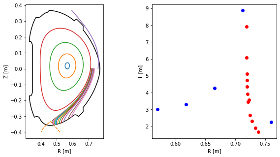
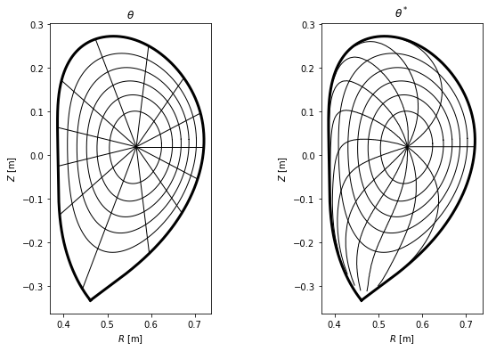
Finally, we plot the difference between the two coordinate systems in the poloidal cross-section view, where lines represent points with constant \(\psi_N\) and \(\theta\) (or \(\theta^*\)).

#Define flux surfaces where theta will be evaluated
psi_n = np.linspace(0, 1, 200)[1:-1]
surfs = [eq._flux_surface(pn)[0] for pn in psi_n]

#Define the flux surfaces which will show on the plot
psi_n2 = np.linspace(0, 1, 7)[1:]
surfs2 = [eq._flux_surface(pn)[0] for pn in psi_n2]

#Define poloidal angles where theta isolines will be plotted
thetas = np.linspace(0, 2*np.pi, 13, endpoint=False)

#Prepare figure
fig, axes = plt.subplots(1, 2, figsize=(10,6))
ax1, ax2 = axes

#Plot LCFS and several flux surfaces in both the plots
eq.lcfs.plot(ax = ax1, color = 'k', ls = '-', lw=3)
eq.lcfs.plot(ax = ax2, color = 'k', ls = '-', lw=3)
for s in surfs2:
    s.plot(ax = ax1, color='k', lw = 1)
    s.plot(ax = ax2, color='k', lw = 1)

#Plot theta and theta_star isolines
for th in thetas:
    # this is so ugly it has to implemented better as soon as possible (!)
#    print(th)
    c = eq.coordinates(r = np.linspace(0, 0.4, 150), theta = np.ones(150)*th)
    amin = np.argmin(np.abs(c.psi_n - 1))
    r_lcfs = c.r[amin]

    psi_n = np.array([np.mean(s.psi_n) for s in surfs])
    c = eq.coordinates(r = np.linspace(0, r_lcfs, len(psi_n)), theta=np.ones(len(psi_n))*th)
    c.plot(ax = ax1, color='k', lw=1)

    idxs = [np.argmin(np.abs(s.straight_fieldline_theta - th)) for s in surfs]
    rs = [s.r[i] for s,i in zip(surfs,idxs)]
    rs = np.hstack((0, rs))
    thetas  = [s.theta[i] for s,i in zip(surfs,idxs)]
    thetas = np.hstack((0, thetas))
    c = eq.coordinates(r = rs, theta = thetas)
    c.plot(ax = ax2, color = 'k', lw=1)

# Make both the subplots pretty
ax1.set_title(r'$\theta$')
ax1.set_aspect('equal')
ax1.set_xlabel('$R$ [m]')
ax1.set_ylabel('$Z$ [m]')
ax2.set_title(r'$\theta^*$')
ax2.set_aspect('equal')
ax2.set_xlabel('$R$ [m]')
ax2.set_ylabel('$Z$ [m]')

Text(0, 0.5, '$Z$ [m]')

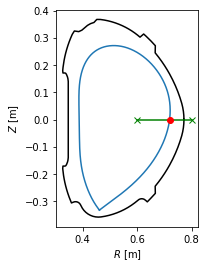
Separatrix position in a profile

In experiment, one is often interested where the separatrix is along the chord of their measurement. In the following example the separatrix coordinates are calculated at the geometric outer midplane, that is, \(Z=0\).

#Define the measurement chord using two points
chord = eq.coordinates(R=[0.6,0.8], Z=[0,0])

#Calculate the intersection of the chord with the separatrix in 2D
intersection_point = chord.intersection(eq.lcfs, dim=2)

#Plot the plasma with the intersection point
ax = plt.gca()
eq.lcfs.plot()
eq.first_wall.plot(c='k')
chord.plot(color='g', marker='x')
intersection_point.plot(marker='o', color='r')
ax.set_aspect('equal')
ax.set_xlabel('$R$ [m]')
ax.set_ylabel('$Z$ [m]')

intersection_point.R

array([0.71882008])