Common PLEQUE tasks

In this notebook, we cover the most common tasks involving a magnetic equilibrium. These are:

• mapping along the magnetic surfaces
• field line tracing
• equilibrium visualisation using contour plots
• individual flux surface examination
• locating the separatrix position in a given profile
• detector line of sight visualisation

%pylab inline

from pleque.io.readers import read_geqdsk
from pleque.utils.plotting import *
from pleque.tests.utils import get_test_equilibria_filenames

Populating the interactive namespace from numpy and matplotlib

Load a testing equilibrium

Several test equilibria come shipped with PLEQUE. Their location is:

gfiles = get_test_equilibria_filenames()
gfiles

['/home/docs/checkouts/readthedocs.org/user_builds/pleque/envs/feature-improve_doc/lib/python3.6/site-packages/pleque/resources/baseline_eqdsk',
 '/home/docs/checkouts/readthedocs.org/user_builds/pleque/envs/feature-improve_doc/lib/python3.6/site-packages/pleque/resources/scenario_1_baseline_upward_eqdsk',
 '/home/docs/checkouts/readthedocs.org/user_builds/pleque/envs/feature-improve_doc/lib/python3.6/site-packages/pleque/resources/DoubleNull_eqdsk',
 '/home/docs/checkouts/readthedocs.org/user_builds/pleque/envs/feature-improve_doc/lib/python3.6/site-packages/pleque/resources/g13127.1050',
 '/home/docs/checkouts/readthedocs.org/user_builds/pleque/envs/feature-improve_doc/lib/python3.6/site-packages/pleque/resources/14068@1130_2kA_modified_triang.gfile',
 '/home/docs/checkouts/readthedocs.org/user_builds/pleque/envs/feature-improve_doc/lib/python3.6/site-packages/pleque/resources/g15349.1120',
 '/home/docs/checkouts/readthedocs.org/user_builds/pleque/envs/feature-improve_doc/lib/python3.6/site-packages/pleque/resources/shot8078_jorek_data.nc']

We store one of the text equilibria in the variable eq, an instance of the Equilibrium class.

test_case_number = 5

#Load equilibrium stored in the EQDSK format
eq = read_geqdsk(gfiles[test_case_number])

#Plot basic overview of the equilibrium
plt.figure()
eq._plot_overview()

#Plot X-points
plot_extremes(eq, markeredgewidth=2)

  nx = 33, ny = 33
361 231
---------------------------------
Equilibrium module initialization
---------------------------------
--- Generate 2D spline ---
--- Looking for critical points ---
--- Recognizing equilibrium type ---
>> X-point plasma found.
--- Looking for LCFS: ---
Relative LCFS error: 2.452534050621385e-12
--- Generate 1D splines ---
--- Mapping midplane to psi_n ---
--- Mapping pressure and f func to psi_n ---

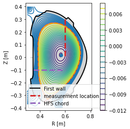
Mapping along the magnetic surfaces

In experiment one often encounters the need to compare profiles which were measured at various locations in the tokamak. In this section, we show how such a profile may be mapped onto an arbitrary location and to the outer midplane.

Our example profile is measured at the plasma top (plotted in red by the following code). It will be mapped to a chord located on the HFS (in violet) and to the outer midplane (not shown in the picture). Note that the outer midplane is defined by the O-point height, not with regard to the chamber (\(Z=0\) etc.).

# Define the chord along which the profile was measured (in red)
N = 200 #number of datapoints in the profile
chord = eq.coordinates(R=0.6*np.ones(N), Z=np.linspace(0.3, 0., N))

# Define the HFS chord where we wish to map the profile (in violet)
chord_hfs = eq.coordinates(R=np.linspace(0.35, 0.6, 20), Z=-0.1*np.ones(20))

# Plot both the chords
plt.figure()
eq._plot_overview()
chord.plot(lw=3, ls='--', color='C3', label='measurement location')
chord_hfs.plot(lw=3, ls='--', color='C4', label='HFS chord')
plt.legend(loc=3)

<matplotlib.legend.Legend at 0x7fe7dadc6f60>

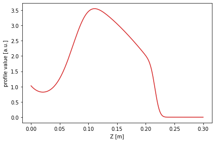
The profile shape is defined somewhat arbitrarily using the error function erf.

from scipy.special import erf

# Define the profile values
prof_func = lambda x, k1, xsep: k1/4 * (1 + erf((x-xsep)*20))*np.log((x+1)*1.2) - 4*np.exp(-(50*(x-1)**2))
profile = prof_func(1 - chord.psi_n, 10, 0.15)

# Plot the profile along the chord where it was measured
plt.figure()
plt.plot(chord.Z, profile, color='C3')
plt.xlabel('Z [m]')
plt.ylabel('profile value [a.u.]')
plt.tight_layout()

To begin the mapping, the profile is converted into a flux function by eq.fluxfuncs.add_flux_func(). The flux function is a spline, and therefore it can be evaluated at any \(\psi_N\) coordinate covered by the original chord. This will allow its mapping to any other coordinate along the flux surfaces.

eq.fluxfuncs.add_flux_func('test_profile', profile, chord, spline_smooth=0)

<scipy.interpolate.fitpack2.InterpolatedUnivariateSpline at 0x7fe7d53a4a90>

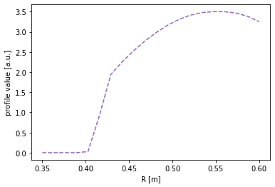
To evaluate the flux function along a chord, simply pass the chord (an instance of the Coordinates class) to the flux function. In the next figure the profile is mapped to the HFS cord.

# Map the profile to the HFS cord
plt.figure()
plt.plot(chord_hfs.R, eq.fluxfuncs.test_profile(chord_hfs), '--', color='C4')
plt.xlabel('R [m]')
plt.ylabel('profile value [a.u.]')

Text(0, 0.5, 'profile value [a.u.]')

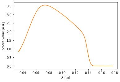
For the outer midplane, no special chord need be specified. Every instance of the Coordinates class can automatically map its coordinates to the outer midplane. (Note that this doesn’t require a flux function to be specified. The conversion is performed in the coordinates only.)

#Map the profile to the outer midplane
plt.figure()
plt.plot(chord.r_mid, profile, color='C1')
plt.xlabel(r'$R$ [m]')
plt.ylabel('profile value [a.u.]')

Text(0, 0.5, 'profile value [a.u.]')

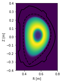
Finally, the profile may be drawn along the entire poloidal cross section.

# Assuming poloidal symmetry, plot the profile in the poloidal cross section
plt.figure()
ax = gca()
ax.plot(eq.lcfs.R, eq.lcfs.Z, color='k', ls='--', lw=2)
ax.plot(eq.first_wall.R, eq.first_wall.Z, 'k-', lw=2)
grid = eq.grid()
ax.pcolormesh(grid.R, grid.Z, eq.fluxfuncs.test_profile(grid))
ax.set_xlabel('R [m]')
ax.set_ylabel('Z [m]')
ax.set_aspect('equal')

Field line tracing

Another task most commonly performed in edge plasma physics is field line tracing and length calculation. (In the core plasma, the field line length is defined as the parallel distance of one poloidal turn. In the SOL, it’s the so-called connection length.)

To showcase field line tracing, first we define a set of five starting points, all located at the outer midplane (\(Z=0\)) with \(R\) going from 0.55 m (core) to 0.76 m (SOL).

# Define the starting points
N = 5
Rs = np.linspace(0.57, 0.76, N, endpoint=True)
Zs = np.zeros_like(Rs)

Next, the field lines beginning at these points are traced. The default tracing direction is direction=1, that is, following the direction of the toroidal magnetic field.

traces = eq.trace_field_line(R=Rs, Z=Zs)

>>> tracing from: 0.570000,0.000000,0.000000
>>> atol = 1e-06
>>> poloidal stopper is used
direction: 1
dphidtheta: 1.0
A termination event occurred., 976
>>> tracing from: 0.617500,0.000000,0.000000
>>> atol = 1e-06
A termination event occurred., 998
>>> tracing from: 0.665000,0.000000,0.000000
>>> atol = 1e-06
A termination event occurred., 1375
>>> tracing from: 0.712500,0.000000,0.000000
>>> atol = 1e-06
A termination event occurred., 3234
>>> tracing from: 0.760000,0.000000,0.000000
>>> atol = 1e-06
The solver successfully reached the end of the integration interval., 35181

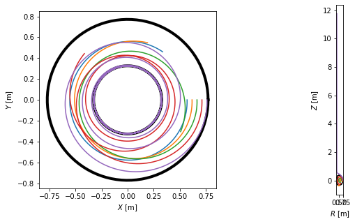
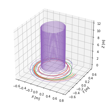
To visualise the field lines, we plot them in top view, poloidal cross-section view and 3D view.

# Define limiter as viewed from the top
Ns = 100
inner_lim = eq.coordinates(np.min(eq.first_wall.R)*np.ones(Ns), np.zeros(Ns), np.linspace(0, 2*np.pi, Ns))
outer_lim = eq.coordinates(np.max(eq.first_wall.R)*np.ones(Ns), np.zeros(Ns), np.linspace(0, 2*np.pi, Ns))

# Create a figure
fig = plt.figure(figsize=(10,5))

# Plot the top view of the field lines
ax = plt.subplot(121)
plt.plot(inner_lim.X, inner_lim.Y, 'k-', lw=4)
plt.plot(outer_lim.X, outer_lim.Y, 'k-', lw=4)
for fl in traces:
    ax.plot(fl.X, fl.Y)
ax.set_xlabel('$X$ [m]')
ax.set_ylabel('$Y$ [m]')
ax.set_aspect('equal')

# Plot the poloidal cross-section view of the field lines
ax = plt.subplot(122)
plt.plot(eq.first_wall.R, eq.first_wall.Z, 'k-')
plt.plot(eq.separatrix.R, eq.separatrix.Z, 'C1--')
for fl in traces:
    plt.plot(fl.R, fl.Z)
ax.set_xlabel('$R$ [m]')
ax.set_ylabel('$Z$ [m]')
ax.set_aspect('equal')

# Plot the 3D view of the field lines
from mpl_toolkits.mplot3d import Axes3D
fig = plt.figure(figsize=(6,6))
ax = fig.gca(projection='3d')
for fl in traces:
    ax.scatter(fl.X, fl.Y, fl.Z, s=0.3, marker='.')
ax.set_xlabel('$X$ [m]')
ax.set_ylabel('$Y$ [m]')
ax.set_zlabel('$Z$ [m]')
#ax.set_aspect('equal')

Text(0.5, 0, '$Z$ [m]')

The field line length may be calculated using its attribute length.

traces[0].length

5.341513172976908

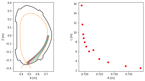
Connection length profile in the SOL

A subtask encountered e.g. in SOL transport analysis is to calculated the connection length \(L\) of a number of SOL flux tubes. To this end, we define a couple more SOL field lines. Note that now the direction argument changes whether we trace to the HFS or LFS limiter/divertor. Also pay attention to the in_first_wall=True argument, which tells the field lines to terminate upon hitting the first wall. (Otherwise they would be terminated at the edge of a rectangle surrounding the vacuum vessel.)

Rsep = 0.7189 # You might want to change this when switching between different test equilibria.
Rs_SOL = Rsep + 0.001*np.array([0, 0.2, 0.5, 0.7, 1, 1.5, 2.5, 4, 6, 9, 15, 20])
Zs_SOL = np.zeros_like(Rs_SOL)

SOL_traces = eq.trace_field_line(R=Rs_SOL, Z=Zs_SOL, direction=-1, in_first_wall=True)

>>> tracing from: 0.718900,0.000000,0.000000
>>> atol = 1e-06
>>> z-lim stopper is used
A termination event occurred., 2296
>>> tracing from: 0.719100,0.000000,0.000000
>>> atol = 1e-06
A termination event occurred., 1664
>>> tracing from: 0.719400,0.000000,0.000000
>>> atol = 1e-06
A termination event occurred., 1504
>>> tracing from: 0.719600,0.000000,0.000000
>>> atol = 1e-06
A termination event occurred., 1426
>>> tracing from: 0.719900,0.000000,0.000000
>>> atol = 1e-06
A termination event occurred., 1305
>>> tracing from: 0.720400,0.000000,0.000000
>>> atol = 1e-06
A termination event occurred., 1226
>>> tracing from: 0.721400,0.000000,0.000000
>>> atol = 1e-06
A termination event occurred., 1093
>>> tracing from: 0.722900,0.000000,0.000000
>>> atol = 1e-06
A termination event occurred., 1006
>>> tracing from: 0.724900,0.000000,0.000000
>>> atol = 1e-06
A termination event occurred., 917
>>> tracing from: 0.727900,0.000000,0.000000
>>> atol = 1e-06
A termination event occurred., 814
>>> tracing from: 0.733900,0.000000,0.000000
>>> atol = 1e-06
A termination event occurred., 719
>>> tracing from: 0.738900,0.000000,0.000000
>>> atol = 1e-06
A termination event occurred., 671

Finally we calculate the connection length and plot its profile.

# Calculate the connection length
L_conn = np.array([SOL_traces[k].length for k in range(len(SOL_traces))])

# Create a figure
fig = plt.figure(figsize=(10,5))

# Plot the poloidal cross-section view of the field lines
ax = plt.subplot(121)
ax.plot(eq.first_wall.R, eq.first_wall.Z, 'k-')
ax.plot(eq.separatrix.R, eq.separatrix.Z, 'C1--')
for fl in SOL_traces:
    ax.plot(fl.R, fl.Z)
ax.set_xlabel('R [m]')
ax.set_ylabel('Z [m]')
ax.set_aspect('equal')

# Plot the connection length profile
ax = plt.subplot(122)
ax.plot(Rs_SOL, L_conn, 'ro')
ax.set_xlabel('R [m]')
ax.set_ylabel('L [m]')

Text(0, 0.5, 'L [m]')

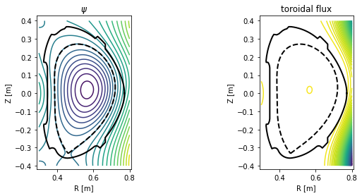
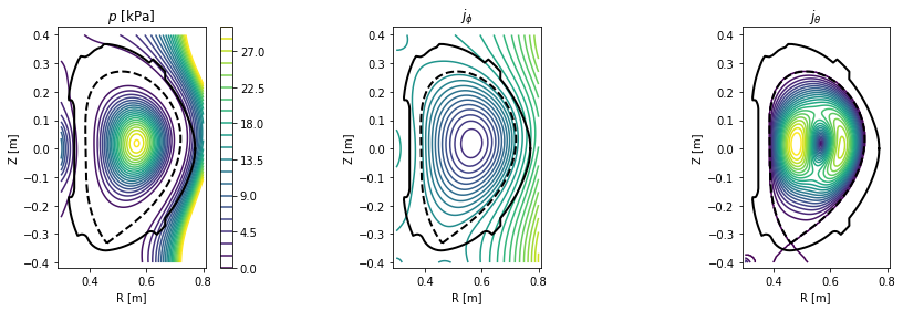
Equilibrium visualisation using contour plots

In this section PLEQUE is used to produce contour plots of the following quantities:

• poloidal magnetic field flux \(\psi\)
• toroidal magnetic field flux
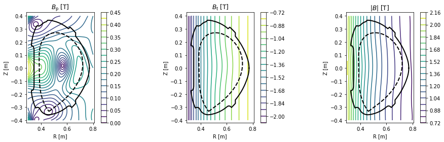
• poloidal magnetic field \(B_p\)
• toroidal magnetic field \(B_t\)
• total magnetic field \(|B|\)
• total pressure \(p\)
• toroidal current density \(j_\phi\)
• poloidal current density \(j_\theta\)

First, a general plotting function plot_2d is defined.

def plot_2d(R, Z, data, *args, title=None):

    # Define X and Y axis limits based on the vessel size
    rlim = [np.min(eq.first_wall.R), np.max(eq.first_wall.R)]
    zlim = [np.min(eq.first_wall.Z), np.max(eq.first_wall.Z)]
    size = rlim[1] - rlim[0]
    rlim[0] -= size / 12
    rlim[1] += size / 12
    size = zlim[1] - zlim[0]
    zlim[0] -= size / 12
    zlim[1] += size / 12

    # Set up the figure: set axis limits, draw LCFS and first wall, write labels
    ax = plt.gca()
    ax.set_xlim(rlim)
    ax.set_ylim(zlim)
    ax.plot(eq.lcfs.R, eq.lcfs.Z, color='k', ls='--', lw=2)
    ax.plot(eq.first_wall.R, eq.first_wall.Z, 'k-', lw=2)
    ax.set_xlabel('R [m]')
    ax.set_ylabel('Z [m]')
    ax.set_aspect('equal')
    if title is not None:
        ax.set_title(title)

    # Finally, plot the desired quantity
    cl = ax.contour(R, Z, data, *args)

    return cl

Next we set up an \([R,Z]\) grid where these quantities are evaluated and plot the quantities.

# Create an [R,Z] grid 200 by 300 points
grid = eq.grid((200,300), dim='size')

# Plot the poloidal flux and toroidal flux
plt.figure(figsize=(16,4))
plt.subplot(131)
plot_2d(grid.R, grid.Z, grid.psi, 20, title=r'$\psi$')
plt.subplot(132)
plot_2d(grid.R, grid.Z, eq.tor_flux(grid), 100, title='toroidal flux')

# Plot the poloidal magnetic field, toroidal magnetic field and the total magnetic field
plt.figure(figsize=(16,4))
plt.subplot(131)
cl = plot_2d(grid.R, grid.Z, eq.B_pol(grid), 20, title=r'$B_\mathrm{p}$ [T]')
plt.colorbar(cl)
plt.subplot(132)
cl = plot_2d(grid.R, grid.Z, eq.B_tor(grid), 20, title=r'$B_\mathrm{t}$ [T]')
plt.colorbar(cl)
plt.subplot(133)
cl = plot_2d(grid.R, grid.Z, eq.B_abs(grid), 20, title=r'$|B|$ [T]')
plt.colorbar(cl)

# Plot the total pressure, toroidal current density and poloidal current density
plt.figure(figsize=(16,4))
plt.subplot(131)
cl = plot_2d(grid.R, grid.Z, eq.pressure(grid)/1e3, np.linspace(0, 30, 21), title=r'$p$ [kPa]')
plt.colorbar(cl)
plt.subplot(132)
plot_2d(grid.R, grid.Z, eq.j_tor(grid), np.linspace(-5e6, 5e6, 30), title=r'$j_\phi$')
plt.subplot(133)
plot_2d(grid.R, grid.Z, eq.j_pol(grid),  np.linspace(0, 3e5, 21), title=r'$j_\theta$')

--- Generating q-splines ---
1%
11%
21%
31%
41%
51%
61%
71%
81%
91%

<matplotlib.contour.QuadContourSet at 0x7fe7d4c7c7b8>

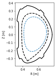
Individual flux surface examination

With the eq._flux_surface(psi_n) function, one may study individual flux surfaces. In this section, we plot the \(\psi_N=0.8\) flux surface and calculate its safety factor \(q\), length in the poloidal direction, total 3D area, volume and toroidal current density.

# Define the flux surface by its normalised poloidal flux
surf = eq._flux_surface(psi_n=0.8)[0]

# Plot the flux surface
plt.figure()
ax = gca()
ax.plot(eq.lcfs.R, eq.lcfs.Z, color='k', ls='--', lw=2)
ax.plot(eq.first_wall.R, eq.first_wall.Z, 'k-', lw=2)
surf.plot(ls='--')
ax.set_xlabel('R [m]')
ax.set_ylabel('Z [m]')
ax.set_aspect('equal')

# Calculate several flux surface quantities
print('Safety factor: %.2f' % surf.eval_q[0])
print('Length: %.2f m' % surf.length)
print('Area: %.4f m^2' % surf.area)
print('Volume: %.3f m^3' % surf.volume)
print('Toroidal current density: %.3f MA/m^2' % (surf.tor_current/1e6))

Safety factor: -1.94
Length: 1.16 m
Area: 0.0989 m^2
Volume: 0.339 m^3
Toroidal current density: -0.213 MA/m^2

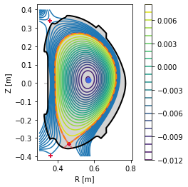
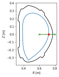
Locating the separatrix position in a given profile

In experiment, one is often interested where the separatrix is along the chord of their measurement. In the following example the separatrix coordinates are calculated at the geometric outer midplane, that is, \(Z=0\).

# Define the measurement chord using two points
chord = eq.coordinates(R=[0.6,0.8], Z=[0,0])

# Calculate the intersection of the chord with the separatrix in 2D
intersection_point = chord.intersection(eq.lcfs, dim=2)

# Plot the plasma with the intersection point
ax = plt.gca()
eq.lcfs.plot()
eq.first_wall.plot(c='k')
chord.plot(color='g', marker='x')
intersection_point.plot(marker='o', color='r')
ax.set_aspect('equal')
ax.set_xlabel('$R$ [m]')
ax.set_ylabel('$Z$ [m]')

intersection_point.R

array([0.71882008])

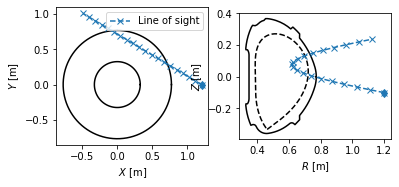
Detector line of sight visualisation

In this section, we demonstrate the flexibility of the Coordinates class by visualising a detector line of sight. Suppose we have a pixel detector at the position \([X, Y, Z] = [1.2 \, \mathrm{m}, 0 \, \mathrm{m}, -0.1 \, \mathrm{m}]\).

# Define detector position [X, Y, Z]
position = np.array((1.2, 0, -0.1))

The detector views the plasma mostly tangentially to the toroidal direction, but also sloping a little upward.

# Define the line of sight direction (again along [X, Y, Z])
direction = np.array((-1, 0.6, 0.2))

# Norm the direction to unit length
direction /= np.linalg.norm(direction)

Now since the plasma geometry is curvilinear, the detector line of sight is not trivial. Luckily PLEQUE’s Coordinates class can easily express its stored coordinates both in the cartesian \([X,Y,Z]\) and the cylindrical \([R,Z,\phi]\) coordinate systems. In the following line, 20 points along the detector line of sight are calculated in 3D.

# Calculate detector line of sight (LOS)
LOS = eq.coordinates(position + direction[np.newaxis,:] * np.linspace(0, 2.0, 20)[:, np.newaxis],
                     coord_type=('X', 'Y', 'Z')
                    )

To visualise the line of sight in top view \([X,Y]\) and poloidal cross-section view \([R,Z]\), we first define the limiter outline as viewed from the top. Then we proceed with the plotting.

# Define the limiter outline as viewed from the top
Ns = 100
inner_lim = eq.coordinates(np.min(eq.first_wall.R)*np.ones(Ns), np.zeros(Ns), np.linspace(0, 2*np.pi, Ns))
outer_lim = eq.coordinates(np.max(eq.first_wall.R)*np.ones(Ns), np.zeros(Ns), np.linspace(0, 2*np.pi, Ns))

# Create a figure
fig, axs = plt.subplots(1,2)

# Plot the top view of the line of sight
ax = axs[0]
ax.plot(inner_lim.X, inner_lim.Y, 'k-')
ax.plot(outer_lim.X, outer_lim.Y, 'k-')
ax.plot(LOS.X, LOS.Y, 'x--', label='Line of sight')
ax.plot(position[0], position[1], 'd', color='C0')
ax.legend()
ax.set_aspect('equal')
ax.set_xlabel('$X$ [m]')
ax.set_ylabel('$Y$ [m]')

# Plot the poloidal cross-section view of the line of sight
ax = axs[1]
ax.plot(eq.first_wall.R, eq.first_wall.Z, 'k-')
ax.plot(eq.lcfs.R, eq.lcfs.Z, 'k--')
ax.plot(LOS.R, LOS.Z, 'x--')
ax.plot(LOS.R[0], position[2], 'd', color='C0')
ax.set_aspect('equal')
ax.set_xlabel('$R$ [m]')
ax.set_ylabel('$Z$ [m]')

Text(0, 0.5, '$Z$ [m]')