PLEQUE vs raw reconstruction

In this notebook, we demonstrate the advantages of using PLEQUE rather than the raw reconstruction data. In particular, we will show the increase of spatial resolution (especially around the X-point) and showcase several methods of \(q\) profile calculation.

%pylab inline

from pleque.io import _geqdsk as eqdsktool
from pleque.io.readers import read_geqdsk
from pleque.utils.plotting import *
from pleque.tests.utils import get_test_equilibria_filenames

Populating the interactive namespace from numpy and matplotlib

Load a testing equilibrium

Several test equilibria come shipped with PLEQUE. Their location is:

gfiles = get_test_equilibria_filenames()
gfiles

['/home/docs/checkouts/readthedocs.org/user_builds/pleque/envs/feature-improve_doc/lib/python3.6/site-packages/pleque/resources/baseline_eqdsk',
 '/home/docs/checkouts/readthedocs.org/user_builds/pleque/envs/feature-improve_doc/lib/python3.6/site-packages/pleque/resources/scenario_1_baseline_upward_eqdsk',
 '/home/docs/checkouts/readthedocs.org/user_builds/pleque/envs/feature-improve_doc/lib/python3.6/site-packages/pleque/resources/DoubleNull_eqdsk',
 '/home/docs/checkouts/readthedocs.org/user_builds/pleque/envs/feature-improve_doc/lib/python3.6/site-packages/pleque/resources/g13127.1050',
 '/home/docs/checkouts/readthedocs.org/user_builds/pleque/envs/feature-improve_doc/lib/python3.6/site-packages/pleque/resources/14068@1130_2kA_modified_triang.gfile',
 '/home/docs/checkouts/readthedocs.org/user_builds/pleque/envs/feature-improve_doc/lib/python3.6/site-packages/pleque/resources/g15349.1120',
 '/home/docs/checkouts/readthedocs.org/user_builds/pleque/envs/feature-improve_doc/lib/python3.6/site-packages/pleque/resources/shot8078_jorek_data.nc']

Load the equilibrium directly

Here the test equilibrium (as it was calculated by EFIT) is directly loaded and stored in the variable eq_efit. The variable then contains all equilibrium information in the form of a dictionary.

test_case_number = 5

with open(gfiles[test_case_number], 'r') as f:
    eq_efit = eqdsktool.read(f)
eq_efit.keys()

  nx = 33, ny = 33
361 231

dict_keys(['nx', 'ny', 'rdim', 'zdim', 'rcentr', 'rleft', 'zmid', 'rmagx', 'zmagx', 'simagx', 'sibdry', 'bcentr', 'cpasma', 'F', 'pres', 'FFprime', 'pprime', 'psi', 'q', 'rbdry', 'zbdry', 'rlim', 'zlim'])

Load equilibrium using PLEQUE

PLEQUE loads the same EFIT output file at its core, but it wraps it in the Equilibrium class and stores it in the variable eq.

#Load equilibrium stored in the EQDSK format
eq = read_geqdsk(gfiles[test_case_number])

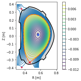
#Plot basic overview of the equilibrium
plt.figure()
eq._plot_overview()

#Plot X-points
plot_extremes(eq, markeredgewidth=2)

  nx = 33, ny = 33
361 231
---------------------------------
Equilibrium module initialization
---------------------------------
--- Generate 2D spline ---
--- Looking for critical points ---
--- Recognizing equilibrium type ---
>> X-point plasma found.
--- Looking for LCFS: ---
Relative LCFS error: 2.452534050621385e-12
--- Generate 1D splines ---
--- Mapping midplane to psi_n ---
--- Mapping pressure and f func to psi_n ---

PLEQUE vs raw reconstruction: increased spatial resolution

EFIT output (\(\Psi\), \(j\) etc.) is given on a rectangular grid. We recreate this grid from the geometric data contained in eq_efit:

r_axis = np.linspace(eq_efit["rleft"], eq_efit["rleft"] + eq_efit["rdim"], eq_efit["nx"])
z_axis = np.linspace(eq_efit["zmid"] - eq_efit["zdim"] / 2, eq_efit["zmid"] + eq_efit["zdim"] / 2, eq_efit["ny"])

To limit the file size, the grid has a finite resolution. This means that in areas where high spatial resolution is needed (for instance the X-point vicinity), raw reconstructions are usually insufficient. The following figure demonstrates this.

# Create a figure
plt.figure()
ax = plt.gca()

# Plot the limiter as stored in EFIT output
ax.plot(eq_efit['rlim'], eq_efit['zlim'], color='k', lw=2)

# Plot the magnetic surface which is defined by Psi == eq_efit['sibdry']
ax.contour(r_axis, z_axis, eq_efit['psi'].T, [eq_efit['sibdry']])

# Plot the magnetic surface saved as the LCFS in EFIT output
ax.plot(eq_efit['rbdry'], eq_efit['zbdry'], 'C0-.', lw=2, label='EFIT LCFS')

# Label the plot and zoom in to the X-point area
ax.set_xlabel('R [m]')
ax.set_ylabel('Z [m]')
ax.set_aspect('equal')
plt.legend()
ax.set_xlim(0.4, 0.54)
ax.set_ylim(-0.38, -0.28)

(-0.38, -0.28)

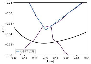
It is apparrent that the raw reconstruction spatial resolution is insufficient, especially when defining magnetic surfaces with a specific value of \(\psi_N\). PLEQUE, on the other hand, performs equilibrium interpolation that can easily produce the same plots with a much higher spatial resolution.

# Create a figure
plt.figure()
ax = plt.gca()

# Plot the limiter (accessed through the Equilibrium class)
eq.first_wall.plot(ls="-", color="k", lw=2)

# Plot the separatrix, cropped to its part inside the first wall
inside_fw = eq.in_first_wall(eq.separatrix)
separatrix = eq.coordinates(R=eq.separatrix.R[inside_fw], Z=eq.separatrix.Z[inside_fw])
separatrix.plot(label='separatrix')

# Plot the LCFS (boundary between the core and the SOL, excluding divertor legs)
eq.lcfs.plot(color='C1', ls='--', label='LCFS')

# Plot the X-point
ax.plot(eq._x_point[0], eq._x_point[1], 'k+', markersize=10, label='X-point')

# Label the plot and zoom in to the X-point area
ax.set_xlabel('R [m]')
ax.set_ylabel('Z [m]')
ax.set_aspect('equal')
plt.legend()
ax.set_xlim(0.4, 0.54)
ax.set_ylim(-0.38, -0.28)

(-0.38, -0.28)

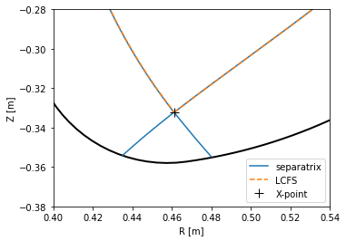
PLEQUE is better suited not only for equilibrium visualisation, but also for calculations based on precise knowledge of the local magnetic field, such as magnetic field line tracing (described in another example notebook).

PLEQUE vs raw reconstruction: \(q\) profile

The safety factor \(q\) can be defined as the number of toroidal turns a magnetic field line makes along its magnetic surface before it makes a full poloidal turn. Since the poloidal field is zero at the X-point, the magnetic field lines on the separatrix surface are caught in an infinite toroidal loop at the X-point and \(q \rightarrow +\infty\). (This is why the edge safety factor is given as \(q_{95}\) at \(\psi_N=0.95\). If it were given an \(\psi_N = 1.00\), its value would diverge regardless of its profile shape.)

In this section we compare several methods of calculating \(q\):

1. \(q\) as calculated by the reconstruction itself (q_efit)
2. \(q\) evaluated by eq.q (q_eq)
3. \(q\) evaluated by eq._flux_surface(psi_n).eval_q
   • using the default, rectangle rule (q1)
   • using the trapezoidal rule (q2)
   • using the Simpson rule (q3)

Method 3 calculates the safety factor according to formula (5.35) in [Jardin, 2010: Computation Methods in Plasma Physics]:

\(q(\psi) = \dfrac{gV'}{(2\pi)^2\Psi'}\langle R^{-2}\rangle\)

where \(V'\) is the differential volume and, in PLEQUE’s notation, \(g(\psi) \equiv F(\psi)\) and \(\Psi \equiv \psi\) (and therefore \(\Psi' \equiv d\Psi/d\psi = 1\)). Furthermore, the surface average \(\langle \cdot \rangle\) of an arbitrary function \(a\) is defined as \(\langle a \rangle = \frac{2\pi}{V'} \int_0^{2\pi} d\theta Ja\) where \(J\) is the Jacobian. Putting everything together, one obtains the formula used by PLEQUE:

\(q(\psi) = \dfrac{F(\psi)}{2\pi} \int_0^{2\pi} d\theta JR^{-2}\)

where, based on the convention defined by COCOS, the factor \(2\pi\) can be missing and \(q\) may be either positive or negative. (In the default convention of EFIT, COCOS 3, \(q\) is negative.) Finally, the integral can be calculated with three different methods: the rectangle rule (resulting in q1), the trapezoidal rule (resulting in q2) and the Simpson rule (resulting in q3).

Method 2 is based on method 3. The safety factor profile is calculated for 200 points in \(\psi_N \in (0, 1)\) and interpolated with a spline. eq.q then invokes this spline to calculate \(q\) at any given \(\psi_N\).

In the following code, we load/calculate the five \(q\) profiles and compare their accuracy.

#Load q taken directly from the reconstruction
q_efit = eq_efit['q']
q_efit = q_efit[:-1] #q is calculated up to psi_N=1, so we exclude this last point
psi_efit = np.linspace(0, 1, len(q_efit), endpoint=False)
#psi_efit2 = np.linspace(0, 1, len(q_efit), endpoint=True)
# If you try this for several test equilibria, you will find that some give q at Psi_N=1
# and some stop right short of Psi_N=1. To test which is which, try both including and
# excluding the endpoint in the linspace definition.

# Calculate q using the Equilibrium class spline
coords = eq.coordinates(psi_n = np.linspace(0, 1, len(q_efit), endpoint=False))
psi_eq = coords.psi_n
q_eq = abs(eq.q(coords))

# Calculate q using eq._flux_surface(Psi).eval_q
surf_psin = linspace(0.01, 1, len(q_efit), endpoint=False)
surfs = [eq._flux_surface(psi_n=psi_n)[0] for psi_n in surf_psin]
surf_psin = [np.mean(s.psi_n) for s in surfs]
q1 = abs(np.array([np.asscalar(s.eval_q) for s in surfs]))
q2 = abs(np.array([np.asscalar(s.get_eval_q('trapz')) for s in surfs]))
q3 = abs(np.array([np.asscalar(s.get_eval_q('simps')) for s in surfs]))

--- Generating q-splines ---
1%
11%
21%
31%
41%
51%
61%
71%
81%
91%

/home/docs/checkouts/readthedocs.org/user_builds/pleque/envs/feature-improve_doc/lib/python3.6/site-packages/ipykernel_launcher.py:19: DeprecationWarning: np.asscalar(a) is deprecated since NumPy v1.16, use a.item() instead
/home/docs/checkouts/readthedocs.org/user_builds/pleque/envs/feature-improve_doc/lib/python3.6/site-packages/ipykernel_launcher.py:20: DeprecationWarning: np.asscalar(a) is deprecated since NumPy v1.16, use a.item() instead
/home/docs/checkouts/readthedocs.org/user_builds/pleque/envs/feature-improve_doc/lib/python3.6/site-packages/ipykernel_launcher.py:21: DeprecationWarning: np.asscalar(a) is deprecated since NumPy v1.16, use a.item() instead

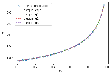
Notice the absolute values in the previous code; this is required because \(q<0\) in the convention used here. We now plot the five \(q\) profiles over each other.

# Create a figure
plt.figure()

# Plot the five q profiles
plt.plot(psi_efit, q_efit, 'x', label='raw reconstruction')
#plt.plot(psi_efit2, q_efit, 'x', label='raw reconstruction')
plt.plot(psi_eq, q_eq, '--', label=r'pleque: eq.q')
plt.plot(surf_psin, q1, '-', label=r'pleque: q1')
plt.plot(surf_psin, q2, '--', label=r'pleque: q2')
plt.plot(surf_psin, q3, '--', label=r'pleque: q3')

# Label the plot and denote the separatrix at Psi_N=1
plt.xlabel(r'$\psi_\mathrm{N}$')
plt.ylabel(r'$q$')
plt.axvline(1, ls='--', color='k', lw=1)
plt.legend()

<matplotlib.legend.Legend at 0x7f05cc4d0b00>

Evidently the five \(q\) profiles are very similar to one another. In the following code we plot their mutual differences. Notice that, using method 3, the \(\psi_N\) axis begins at 0.01 and not 0. This is because \(q\) cannot be calculated by the formula above in \(\psi_N=0\) and the algorithm fails.

# Create a figure
plt.figure(figsize=(12,4))

# Plot EFIT vs eq.q
plt.subplot(121)
plt.plot(surf_psin, abs(q_eq-q_efit), label='EFIT vs eq.q')
plt.legend()
plt.xlabel(r'$\psi_\mathrm{N}$')
plt.ylabel(r'$\Delta q$')

# Plot EFIT vs q1-q3
plt.subplot(122)
plt.plot(surf_psin, abs(q_efit-q1), label='EFIT vs q2')
plt.plot(surf_psin, abs(q_efit-q2), label='EFIT vs q3')
plt.plot(surf_psin, abs(q_efit-q3), label='EFIT vs q3')
plt.legend()
plt.xlabel(r'$\psi_\mathrm{N}$')
plt.ylabel(r'$\Delta q$')

# Create another figure
plt.figure(figsize=(12,4))

# Plot eq.q vs all the rest
plt.subplot(121)
plt.plot(surf_psin, abs(q_eq-q1), label='eq.q vs q1')
plt.plot(surf_psin, abs(q_eq-q2), label='eq.q vs q2')
plt.plot(surf_psin, abs(q_eq-q3), label='eq.q vs q3')
plt.legend()
plt.xlabel(r'$\psi_\mathrm{N}$')
plt.ylabel(r'$\Delta q$')

#Plot q1 vs q2 vs q3
plt.subplot(122)
plt.plot(surf_psin, abs(q1-q2), label='q1 vs q2')
plt.plot(surf_psin, abs(q1-q3), label='q1 vs q3')
plt.plot(surf_psin, abs(q2-q3), label='q2 vs q3')
plt.legend()
plt.xlabel(r'$\psi_\mathrm{N}$')
plt.ylabel(r'$\Delta q$')

Text(0, 0.5, '$\\Delta q$')

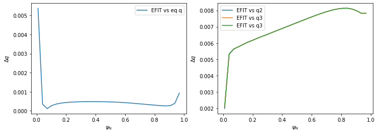
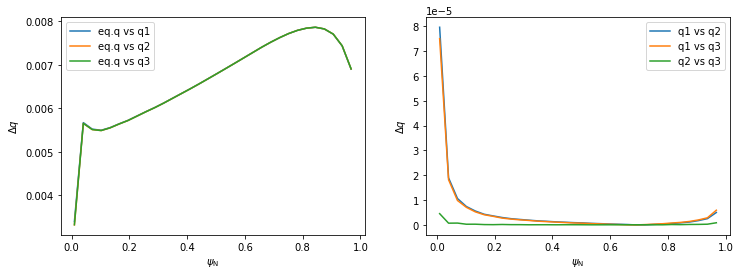
The profiles disagree slightly near \(\psi_N \rightarrow 0\) since the safety factor is defined by a limit here. For the most part, however, PLEQUE and raw reconstcruction values of \(q\) match quite well. PLEQUE can therefore be used to fill in the space between the EFIT datapoint, which can be useful especially near the separatrix where \(q\) rises sharply.