Straight field lines

This example notebook contains a playful exercise with PLEQUE: exploring an unusual coordinate system \([R, \theta^*, \phi]\) where, unlike in regular toroidal coordinates \([R, \theta, \phi]\), magnetic field lines are straight. This exercise is not particularly useful for everyday life (perhaps save for a few niche MHD uses), but it illustrates the flexibility and power of PLEQUE for various equilibrium-related tasks.

%pylab inline

from pleque.io.readers import read_geqdsk
from pleque.utils.plotting import *
from pleque.tests.utils import get_test_equilibria_filenames

Populating the interactive namespace from numpy and matplotlib

Load a testing equilibrium

Several test equilibria come shipped with PLEQUE. Their location is:

gfiles = get_test_equilibria_filenames()
gfiles

['/home/docs/checkouts/readthedocs.org/user_builds/pleque/envs/feature-improve_doc/lib/python3.6/site-packages/pleque/resources/baseline_eqdsk',
 '/home/docs/checkouts/readthedocs.org/user_builds/pleque/envs/feature-improve_doc/lib/python3.6/site-packages/pleque/resources/scenario_1_baseline_upward_eqdsk',
 '/home/docs/checkouts/readthedocs.org/user_builds/pleque/envs/feature-improve_doc/lib/python3.6/site-packages/pleque/resources/DoubleNull_eqdsk',
 '/home/docs/checkouts/readthedocs.org/user_builds/pleque/envs/feature-improve_doc/lib/python3.6/site-packages/pleque/resources/g13127.1050',
 '/home/docs/checkouts/readthedocs.org/user_builds/pleque/envs/feature-improve_doc/lib/python3.6/site-packages/pleque/resources/14068@1130_2kA_modified_triang.gfile',
 '/home/docs/checkouts/readthedocs.org/user_builds/pleque/envs/feature-improve_doc/lib/python3.6/site-packages/pleque/resources/g15349.1120',
 '/home/docs/checkouts/readthedocs.org/user_builds/pleque/envs/feature-improve_doc/lib/python3.6/site-packages/pleque/resources/shot8078_jorek_data.nc']

We store one of the text equilibria in the variable eq, an instance of the Equilibrium class.

test_case_number = 5

#Load equilibrium stored in the EQDSK format
eq = read_geqdsk(gfiles[test_case_number])

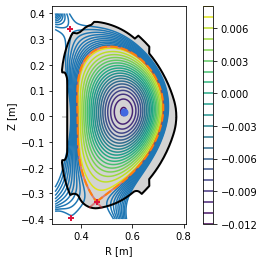
#Plot basic overview of the equilibrium
plt.figure()
eq._plot_overview()

#Plot X-points
plot_extremes(eq, markeredgewidth=2)

  nx = 33, ny = 33
361 231
---------------------------------
Equilibrium module initialization
---------------------------------
--- Generate 2D spline ---
--- Looking for critical points ---
--- Recognizing equilibrium type ---
>> X-point plasma found.
--- Looking for LCFS: ---
Relative LCFS error: 2.452534050621385e-12
--- Generate 1D splines ---
--- Mapping midplane to psi_n ---
--- Mapping pressure and f func to psi_n ---

Define the \(q=5/3\) resonant flux surface

We are going to demonstrate the two coordinate systems on a particular field line: one lying on the resonant surface \(q=5/3\) (therefore it closes upon itself after three poloidal turns). First, we find the \(\Psi_N\) of this surface.

from scipy.optimize import brentq

# Find the Psi_N where the safety factor is 5/3
psi_onq = brentq(lambda psi_n: np.abs(eq.q(psi_n)) - 5/3, 0, 0.95)
print(r'Psi_N = {:.3f}'.format(psi_onq))

--- Generating q-splines ---
1%
11%
21%
31%
41%
51%
61%
71%
81%
91%
Psi_N = 0.714

Next we store this flux surface in the surf variable and define the straight field line coordinate system using its attributes.

from scipy.interpolate import CubicSpline
from numpy import ma #module for masking arrays

#Define the resonant flux surface using its Psi_N
surf = eq._flux_surface(psi_n = psi_onq)[0]

# Define the normal poloidal coordinate theta (and subtract 2*pi from any value that exceeds 2*pi)
theta = np.mod(surf.theta, 2*np.pi)

# Define the special poloidal coordinate theta_star and
theta_star = surf.straight_fieldline_theta

# Sort the two arrays to start at theta=0 and decrease their spatial resolution by 75 %
asort = np.argsort(theta)
#should be smothed
theta = theta[asort][2::4]
theta_star = theta_star[asort][2::4]

# Interpolate theta_star with a periodic spline
thstar_spl = CubicSpline(theta, theta_star, extrapolate='periodic')

Trace a magnetic field line within the \(q=5/3\) resonant flux surface

Now we trace a field line along the resonant magnetic surface, starting at the outer midplane (the intersection of the resonant surface with the horizontal plane passing through the magnetic axis). Since the field line is within the confined plasma, the tracing terminates after one poloidal turn. We begin at the last point of the field line and restart the tracing two more times, obtaining a full field line which closes into itself.

tr1 = eq.trace_field_line(r=eq.coordinates(psi_onq).r_mid[0], theta=0)[0]
tr2 = eq.trace_field_line(tr1.R[-1], tr1.Z[-1], tr1.phi[-1])[0]
tr3 = eq.trace_field_line(tr2.R[-1], tr2.Z[-1], tr2.phi[-1])[0]

>>> tracing from: 0.691640,0.018568,0.000000
>>> atol = 1e-06
>>> poloidal stopper is used
direction: 1
dphidtheta: 1.0
A termination event occurred., 41726
>>> tracing from: 0.691584,0.017475,-209.396043
>>> atol = 1e-06
>>> poloidal stopper is used
direction: 1
dphidtheta: 1.0
A termination event occurred., 2064
>>> tracing from: 0.691638,0.018568,-198.931515
>>> atol = 1e-06
>>> poloidal stopper is used
direction: 1
dphidtheta: 1.0
A termination event occurred., 2068

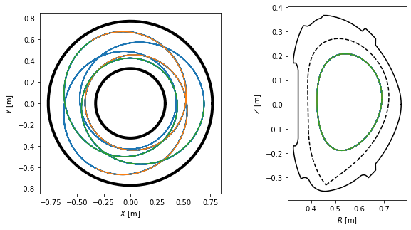
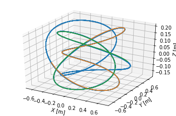
We visualise the three field line parts in top view, poloidal cross-section view and 3D view. Notice that they make five toroidal turns until they close in on themselves, which corresponds to the \(m=5\) resonant surface.

# Create a figure
plt.figure(figsize=(10,5))

# Define the limiter as viewed from the top
Ns = 100
inner_lim = eq.coordinates(np.min(eq.first_wall.R)*np.ones(Ns), np.zeros(Ns), np.linspace(0, 2*np.pi, Ns))
outer_lim = eq.coordinates(np.max(eq.first_wall.R)*np.ones(Ns), np.zeros(Ns), np.linspace(0, 2*np.pi, Ns))

# Plot the field line in the top view
ax = plt.subplot(121)
ax.plot(inner_lim.X, inner_lim.Y, 'k-', lw=4)
ax.plot(outer_lim.X, outer_lim.Y, 'k-', lw=4)
ax.plot(tr1.X, tr1.Y)
ax.plot(tr2.X, tr2.Y)
ax.plot(tr3.X, tr3.Y)
ax.set_xlabel('$X$ [m]')
ax.set_ylabel('$Y$ [m]')
ax.set_aspect('equal')

# Plot the field line in the poloidal cross-section view
ax = plt.subplot(122)
ax.plot(eq.first_wall.R, eq.first_wall.Z, 'k-')
ax.plot(eq.lcfs.R, eq.lcfs.Z, 'k--')
ax.plot(tr1.R, tr1.Z)
ax.plot(tr2.R, tr2.Z)
ax.plot(tr3.R, tr3.Z)
ax.set_xlabel('$R$ [m]')
ax.set_ylabel('$Z$ [m]')
ax.set_aspect('equal')

# Plot the field line in 3D
from mpl_toolkits.mplot3d import Axes3D
fig = plt.figure()
ax = fig.gca(projection='3d')
ax.plot(tr1.X, tr1.Y, tr1.Z)
ax.plot(tr2.X, tr2.Y, tr2.Z)
ax.plot(tr3.X, tr3.Y, tr3.Z)
#ax.set_aspect('equal')
ax.set_xlabel('$X$ [m]')
ax.set_ylabel('$Y$ [m]')
ax.set_zlabel('$Z$ [m]')

Text(0.5, 0, '$Z$ [m]')

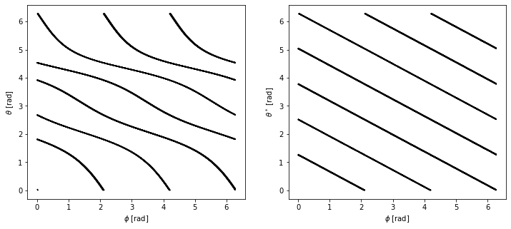
Plot the field line in both coordinate systems

Plotting the field lines in the \([\theta, \phi]\) and \([\theta^*, \phi]\) coordinates, we find that they are curves in the former and straight lines in the latter.

# Create a figure
fig, axes = plt.subplots(1, 2, figsize=(12,5))
ax1, ax2 = axes

for t in [tr1, tr2, tr3]:
    # Extract the theta, theta_star and Phi coordinates from the field lines
    theta = np.mod(t.theta, 2*np.pi)
    theta_star = thstar_spl(theta)
    phi = np.mod(t.phi, 2*np.pi)

    # Mask the coordinates for plotting purposes
    theta = ma.masked_greater(theta, 2*np.pi-1e-2)
    theta = ma.masked_less(theta, 1e-2)
    theta_star = ma.masked_greater(theta_star, 2*np.pi-1e-2)
    theta_star = ma.masked_less(theta_star, 1e-2)
    phi = ma.masked_greater(phi, 2*np.pi-1e-2)
    phi = ma.masked_less(phi, 1e-2)

    # Plot the coordinates [theta, Phi] and [theta_star, Phi]
    ax1.plot(phi, theta, 'k-')
    ax2.plot(phi, theta_star, 'k-')

# Label the two subplots
ax1.set_xlabel(r'$\phi$ [rad]')
ax1.set_ylabel(r'$\theta$ [rad]')
ax2.set_xlabel(r'$\phi$ [rad]')
ax2.set_ylabel(r'$\theta^*$ [rad]')

Text(0, 0.5, '$\\theta^*$ [rad]')

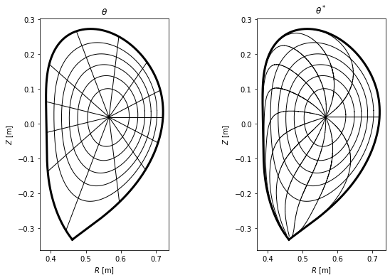
Plot the two coordinate systems in the poloidal cross-section view

Finally, we plot the difference between the two coordinate systems in the poloidal cross-section view, where lines represent points with constant \(\psi_N\) and \(\theta\) (or \(\theta^*\)).

# Define the flux surfaces where theta will be evaluated
psi_n = np.linspace(0, 1, 1000)[1:-1]
surfs = [eq._flux_surface(pn)[0] for pn in psi_n]

# Define the flux surfaces which will show on the plot
psi_n2 = np.linspace(0, 1, 7)[1:]
surfs2 = [eq._flux_surface(pn)[0] for pn in psi_n2]

# Define the poloidal angles where theta isolines will be plotted
thetas = np.linspace(0, 2*np.pi, 13, endpoint=False)

# Create a figure
fig, axes = plt.subplots(1, 2, figsize=(10,6))
ax1, ax2 = axes

# Plot the LCFS and several flux surfaces in both the plots
eq.lcfs.plot(ax = ax1, color = 'k', ls = '-', lw=3)
eq.lcfs.plot(ax = ax2, color = 'k', ls = '-', lw=3)
for s in surfs2:
    s.plot(ax = ax1, color='k', lw = 1)
    s.plot(ax = ax2, color='k', lw = 1)

# Plot the theta and theta_star isolines
for th in thetas:
    # this is so ugly it has to implemented better as soon as possible (!)
#    print(th)
    c = eq.coordinates(r = np.linspace(0, 0.4, 300), theta = np.ones(300)*th)
    amin = np.argmin(np.abs(c.psi_n - 1))
    r_lcfs = c.r[amin]

    psi_n = np.array([np.mean(s.psi_n) for s in surfs])
    c = eq.coordinates(r = np.linspace(0, r_lcfs, len(psi_n)), theta=np.ones(len(psi_n))*th)
    c.plot(ax = ax1, color='k', lw=1)

    idxs = [np.argmin(np.abs(s.straight_fieldline_theta - th)) for s in surfs]
    rs = [s.r[i] for s,i in zip(surfs,idxs)]
    rs = np.hstack((0, rs))
    thetas  = [s.theta[i] for s,i in zip(surfs,idxs)]
    thetas = np.hstack((0, thetas))
    c = eq.coordinates(r = rs, theta = thetas)
    c.plot(ax = ax2, color = 'k', lw=1)

# Label both the subplots
ax1.set_title(r'$\theta$')
ax1.set_aspect('equal')
ax1.set_xlabel('$R$ [m]')
ax1.set_ylabel('$Z$ [m]')
ax2.set_title(r'$\theta^*$')
ax2.set_aspect('equal')
ax2.set_xlabel('$R$ [m]')
ax2.set_ylabel('$Z$ [m]')

Text(0, 0.5, '$Z$ [m]')